Project Ava: On the Matter of Using Machine Learning for Web Application Security Testing – Part 6: Development of Prototype #2 – Creating a SQLi PoC

Following on from the team’s first prototype, which explored text processing and semantic relationships, the sixth blog in the Project Ava series moves on to creating a SQLi proof of concept…

Overview

Building on our initial work with word vectorisation and support-vector machines (SVMs), we set out to create a Proof of Concept (PoC) system capable of detecting potential SQL injection (SQLi) issues affecting a web application, based on properties of HTTP responses. Specifically, we set out to use real-world data for this PoC, moving away from the synthetic data used in our previous experiments. The following approach was followed:

• Real data – a number of known vulnerable web applications were downloaded and tested for SQLi issues. Errors associated with potential SQLi were then uploaded to our elasticsearch server
• Create a Virtual Machine (VM) for ML model generation and manipulation – a Debian VM was created and installed with a number of tools/libraries allowing for ML model generation and manipulation
• Create, train and improving our model – using the data stored in our elasticsearch instance to create datasets and apply NLP algorithms for performing SQLi predictions
• Usage of the model – Using the model, develop a system that would enable its simple usage, involving the creation of easy-to-use Burp plugins and extensions

In this blog we walk through our actual setup of a working environment so that others can try similar experiments and build upon this particular approach.

Collecting real-world vulnerability data

A number of vulnerable web applications were used to collect data that would be useful in creating and training a ML model capable of identifying potential SQLi issues. The following web applications were initially used for this purpose:

• bwapp - bWAPP PHP/MySQL [1]
• webgoat7 - WebGoat 7.1 OWASP Flagship Project [2]
• webgoat8 - WebGoat 8.0 OWASP Flagship Project [2]
• dvwa - Damn Vulnerable Web Application [3]
• mutillidae - OWASP Mutillidae II [4]
• juiceshop - OWASP Juice Shop [5]
• vulnerablewordpress - WPScan Vulnerable Wordpress [6]
• securityninjas - OpenDNS Security Ninjas [7]

For consistency we decided to collect SQLi (error) samples generated by the web applications based on MySQL only. As such only the following applications were based on this particular database management system (DBMS):

• Bwapp
• Dvwa
• Mutillidae
• Vulnerablewordpress

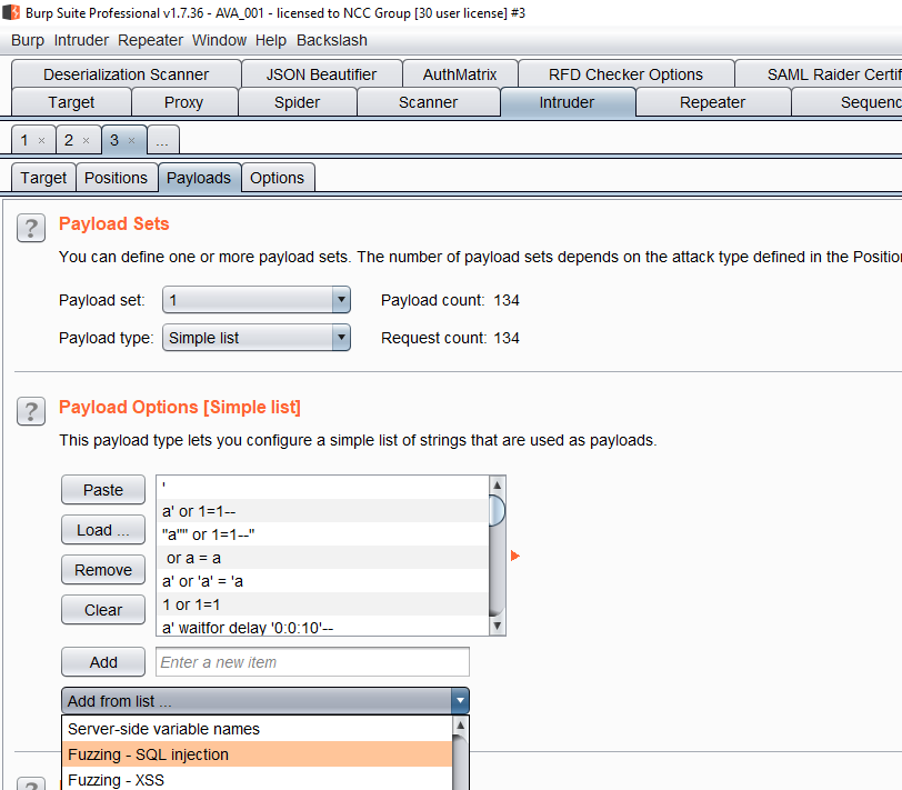
All web traffic to and from these applications was proxied through BurpSuite. The Intruder tool was then used to fuzz the vulnerable fields using the “Fuzzing – SQL injection” payloads available within Burp:

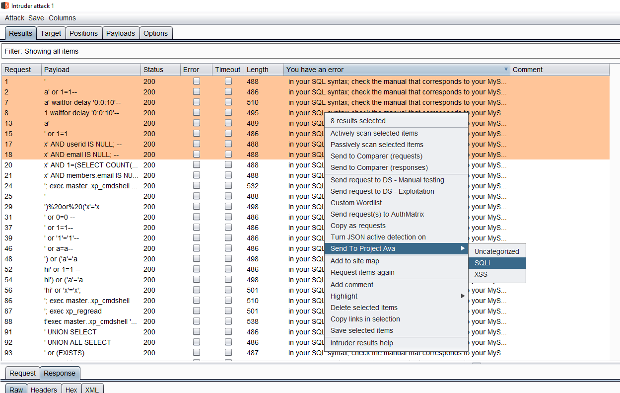
The error samples were then uploaded to our internal elasticsearch server using our Project Ava plugin (see Part 4 of this blog series), which allowed us to classify the confirmed vulnerabilities as SQLi:

A sample of over 1,200 tagged SQLi records was collected. It was also necessary to upload several additional records corresponding to responses that were not SQLi issues. This data was labelled as “non-SQLi” and for consistency only the records that were not producing an error (using the fuzzing technique indicated above) were uploaded.

Creating a VM for ML manipulation

A VM image based on Debian Jessie 8.10 (64 bit) was downloaded from Osboxes.org [8] and used as the base to create a suitable machine for our ML experiments. A number of configuration changes were performed to install Python libraries and the “virtualenv” tool.

A virtual environment (named ava1) was created; below is a list of the python3 modules that were available (note that the packages highlighted in yellow are those that were installed using the “pip install <packagename>” syntax – all additional packages were automatically added by “pip” to satisfy dependencies):

(ava1)osboxes@osboxes:~/ava1$ pip list
Package Version
------------------- -------
absl-py 0.3.0 
astor 0.7.1 
backcall 0.1.0 
backports-abc 0.5 
bleach 2.1.3 
decorator 4.3.0 
entrypoints 0.2.3 
gast 0.2.0 
grpcio 1.14.0 
h5py 2.8.0 
html5lib 1.0.1 
ipykernel 4.8.2 
ipython 6.5.0 
ipython-genutils 0.2.0 
ipywidgets 7.4.0 
jedi 0.12.1 
Jinja2 2.10 
jsonschema 2.6.0 
jupyter 1.0.0 
jupyter-client 5.2.3 
jupyter-console 5.2.0 
jupyter-core 4.4.0 
Keras 2.2.2 
Keras-Applications 1.0.4 
Keras-Preprocessing 1.0.2 
Markdown 2.6.11 
MarkupSafe 1.0 
mistune 0.8.3 
nbconvert 5.3.1 
nbformat 4.4.0 
notebook 5.6.0 
numpy 1.15.0 
pandas 0.23.4 
pandocfilters 1.4.2 
parso 0.3.1 
pexpect 4.6.0 
pickleshare 0.7.4 
pip 18.0 
prometheus-client 0.3.1 
prompt-toolkit 1.0.15 
protobuf 3.6.0 
ptyprocess 0.6.0 
Pygments 2.2.0 
python-dateutil 2.7.3 
pytz 2018.5 
PyYAML 3.13 
pyzmq 17.1.0 
qtconsole 4.3.1 
scikit-learn 0.19.2 
scipy 1.1.0 
Send2Trash 1.5.0 
setuptools 40.0.0 
simplegeneric 0.8.1 
six 1.11.0 
tensorboard 1.9.0 
tensorflow 1.9.0 
termcolor 1.1.0 
terminado 0.8.1 
testpath 0.3.1 
tornado 5.1 
traitlets 4.3.2 
typing 3.6.4 
wcwidth 0.1.7 
webencodings 0.5.1 
Werkzeug 0.14.1 
wheel 0.31.1 
widgetsnbextension 3.4.0 
(ava1)osboxes@osboxes:~/ava1$

Only the following packages/libraries were used to develop our proof of concept model:

• Numpy
• Pandas
• Scipy
• Scikit-learn
• jupyter

Jupyter Notebooks

The “jupyter” package included in the list above was available and permitted the launching of a notebook server. The following command was used to launch it:

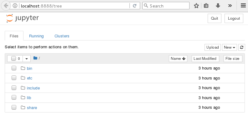
The Jupyter network configuration was changed to allow access from outside the VM. Specifically the following configuration file was changed:

/home/osboxes/.jupyter/jupyter_notebook_config.py

The highlighted change in the configuration line below allowed access from the network:

# Use '*' to allow any origin to access your server.
c.NotebookApp.ip = '*'

Note that in order to connect with the VM from an external network a special token is necessary to use in web requests to the notebook web server. This token can be taken from the output produced by the “jupyter notebook” command on the VM. An example of this token is included below:

$ jupyter notebook list
Currently running servers:
http://localhost:8888/?token=b219e55965fa81c1029c1a827c765a2f2507d32bf5da0a76 :: /home/osboxes

Additional Packages

No additional packages were installed. However we note that a number of modifications were necessary in order to properly use the scikit-learn library. In particular, the following commands were executed to complete a successful installation:

#prerequisites
sudo apt-get install build-essential python3-dev python3-setuptools python3-numpy python3-scipy python3-pip libatlas-dev libatlas3gf-base

#install the actual library
pip3 install scikit-learn

#additional necessary commands
$update-alternatives --set libblas.so.3 /usr/lib/atlas-base/atlas/libblas.so.3

$update-alternatives --set liblapack.so.3 /usr/lib/atlas-base/atlas/liblapack.so.3

Creating and training the ML model

One of the most promising models from Prototype #1 was the SVM-Multiclass. We chose to reuse the code from that previous research (also taken from a Jupyter notebook) to generate a model using the data that we’d captured, labelled and stored in our elasticsearch instance. 

To show our intended approach here, an initial quick proof of concept to use this model can be seen in the code below; in this case a random sample is collected from the available data and submitted to the model which then prints the words “Found potential issue!” when a potential SQLi is identified:

# randomly selecting X_test and performing a prediction
# if SQLi then pring the sample to confirm


import random


total_x=len(X)


print("Total number of data samples: %s" % total_x)


random_row=random.randint(0,total_x-1)


print("Sample #%s selected for prediction." % random_row)


samples=np.array([X[random_row]])
result=text_clf_svm.predict(samples)
print("Result is: %s" % result[0])


#result will include only 1 result
if result[0]=='SQLi':
 print("Found potential issue!")

This approach could be reused in a program fuzzing a specific web application and sending each HTTP response to the model for evaluation. The parameter that should be passed by the fuzzer to this ML model is that of a variable replacing the text highlighted in red above.
As an example the code above could be simplified as follows:

samples=np.array([request_response_data])
result=text_clf_svm.predict(samples)
print("Result is: %s" % result[0])


#result will include only 1 result
if result[0]=='SQLi':
 print("Found potential issue!")

Note that in the code above, the ‘request_response_data’ variable would be set by the fuzzing program.

Improving the model – re-labelling false positives

We observed that the initial model would produce a large amount of false positives when testing web applications that were “not involved” with the model training process (i.e. web applications with requests/responses outside the training datasets). We postulated that the model could be improved through continued testing (fuzzing) of new web applications and sending all false positives to the elasticsearch server marking the records as “non-sqli” - the model would be then re-trained using the new data. This process could be repeated multiple times until the volume of false positives produced becomes tolerable.

This simple algorithm to improve the model can be summarised in the following steps:

1. Test a new application using the ML system
2. Select all false positives and send them to elasticsearch marking them as “non-SQLi”
3. Re-train the model based on the new data
4. Go back to testing the application in 1. to determine if false positives are reduced
5. Continue with testing new applications and repeat from steps 2. onwards

We note however that this process cannot guarantee that the model will be “perfect” at some epoch since the number of web applications available on the Internet, and the number of potential web application code manifestations, is seemingly infinite.

Improving the model – playing with CountVectorizer (CVec) parameters

We investigated finding a good combination of CountVectorizer parameters that would minimise false positives, but this would require the presence of a very large dataset of training data.

Other interesting parameters are that we investigated include:

• max_df - to ignore terms that are repeated too often in the corpus of data (‘corpus specific stop words’)
• ngram_range - to set a range of term combinations based on all the terms included in the corpus

The original model, based on CountVectorizer with stop words, was scoring the following (after increasing the training data to over 8,600 records):

Score for this model: 0.9919608528486543

A new variant of this model using the “max_df” initialization parameter set to 0.1 was then created and fitted using the following code:

cvec1=CountVectorizer(stop_words='english',max_df=0.1)#,max_features=2000)
cvec1.fit(X_train,y_train)

This model was slightly better than the previous one, scoring the following:

Score for this model: 0.9930094372596994

An additional model was then created adding the “ngram_range” option as can be seen within the code below:

cvec2=CountVectorizer(stop_words='english',ngram_range=(2,2),max_df=0.1)
cvec2.fit(X_train,y_train)

This introduced a further improvement in the model score:

Score for this model: 0.9972037749038798

At this point we wanted to test the three models using text from the training data plus additional text that could induce a false positive result. The following code was used as an example:

samples=[]
samples.append(a)
samples.append(b)
#print(samples)
c='''You have an error in your brain'''
samples.append(c)

samples=np.array(samples)
samples.shape
result=text_clf_svm.predict(samples)

print(result)

In the code above ‘a’ was request and response data, with the response including an error message indicating that the web application was potentially affected by SQLi issues. ‘B’ was request and response data not including errors indicating SQL injection problems. Finally, the string ‘c’ was an arbitrary string with a phrase structure similar to that of a MySQL error (i.e. ‘You have an error in your SQL…’).

The first model predicted the following for ‘a’, ‘b’ and ‘c’:

[u'SQLi' u'non SQLi' u'SQLi']

As can be seen ‘a’ was correctly detected, ‘b’ was not a SQLi issue (as expected) and ‘c’ was a false positive.

The same code was then used with a model generated by starting from ‘cvec1’. This model predicted the following:

[u'SQLi' u'non SQLi' u'non SQLi']

As can be seen the string in ‘c’ was not marked as a SQLi issue meaning that this model would be (potentially) less affected by false positives.

Note that the third model (i.e. the one using ‘cvec2’) was also ignoring the string ‘c’, marking it as ‘non SQLi’; this could suggest that the ‘max_df’ parameter, shared by both models, would be beneficial against false positives.

A new model was then generated using just the “ngram_range” option:

cvec3=CountVectorizer(stop_words='english',ngram_range=(2,2))
cvec3.fit(X_train,y_train)

This new model scored as follows:

Score for this model: 0.9947570779447745

As can be seen this model had a score better than the model using only the ‘max_df’ option but a worse score than the model using both options (‘max_df’ plus ‘ngram_range’). When testing this model against the three samples discussed above the following results were produced:

[u'SQLi' u'non SQLi' u'non SQLi']

We see that the model is still ‘good’ at ignoring false positives.

The model with the highest score (using ‘cvec2’) was then pickled and tested with Burp. The model in this case was a 2.4MB file which was detecting SQLi issues in common vulnerable applications although it was observed to be more selective and failing to mark some responses as potentially vulnerable.

Using the ML model

Further actions were necessary in order to use the ML model that was created, as discussed above. Specifically, we wanted to have a system (or process) in place that would allow a consultant using the ML model for prediction without them having to go through the entire process of training and fitting the model. In short a standard solution was implemented that would let an NCC Group consultant use the model simply by having the right libraries installed as part of their Python installation.

Serializing the model to a file

The pickle library can be used to serialize the trained model to a file. This is a simple process as can be seen in the code below; note that the variable highlighted in red is the actual Python object representing the model at run-time:

# code to store the model to a file for later reuse
import pickle
filename = 'sqlizzing_finalized_model.sav'
pickle.dump(text_clf_svm, open(filename, 'wb'))

The file can then be copied to a different machine in order to be used. Note that a number of prerequisites are necessary for this to work on an external machine, as presented below.

Prerequisites to reuse the serialized model

The following prerequisites are necessary to be able to reuse an ML model created as above:

• Python 2.7.x or 3.3 or later
• Numpy 1.15.0
• Scipy 1.1.0
• Scikit-learn 0.19.2

Note that Numpy/Scipy and Scikit-learn could simply be installed using pip:

$> pip install numpy

Testing the model

The model can be used as soon as the prerequisites listed above are satisfied. The following code could be used as an example; this assumes a file representing a serialized version of the model is present in the folder when the Python program below is executed:

# load a ML model from a file
import pickle
filename = 'sqlizzing_finalized_model.sav'
loaded_model = pickle.load(open(filename, 'rb'))

print("model loaded")

# using the loaded model
import numpy as np

a="A request/response whatever"
b="Some random test asdkljadja askdaskd ieqrje9 md,mcd,m 9odkeklm d,fd,f,dfm s3003r033"
c="You have an"
d="You have an error"

samples=[]
samples.append(a)
samples.append(b)
samples.append(c)
samples.append(d)

samples=np.array(samples)
samples.shape

result=loaded_model.predict(samples)

print(result)

A sample result (prediction) of this elaboration is:

['non SQLi' 'SQLi' 'non SQLi' 'SQLi']

A standalone program or plugin could therefore be created to fuzz a web application, using the model for predicting if the target application is potentially affected by SQLi issues.

A Burp extension using the model

Since the ML model is easily exportable to a different system, we decided to develop a Burp extension to interact with it. This Burp extension is based on the same concept of fuzzing that was followed while collecting and categorising data for our elasticsearch instance.

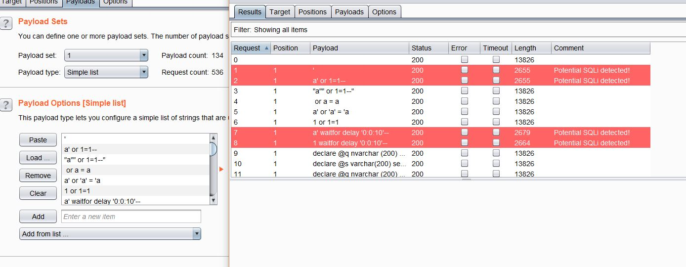
In fact, the main algorithm upon which this extension is based assumes that a tester is performing fuzzing using Burp intruder. Each HTTP message generated by Intruder (including request and response) would then be used to generate testing data to be evaluated by the model. However, we note that the Jython interpreter used by Burp Suite, allowing the creation of extensions written in Python, would not be able to interact with the various ML libraries used by the ML model at runtime.

A workaround to this was to create a simple HTTP server handling POST requests generated by Burp (i.e. POST requests generated with the Intruder data) which are then used as the input data for a prediction. This server would then return a response indicating whether each Intruder message resulted in a potential SQL injection. A screenshot of this plugin in action can be see below:

Summary

In this post we showed a proof of concept model and approach to its training, capable of detecting SQLi issues in web applications with fairly high accuracy. However, a number of caveats were present which curtailed our celebrations, including:

• Data volume – we were still working on comparatively small volumes of data
• Specific DBMS – we had focused on one specific DBMS only (MySQL)
• Re-training – the model would need periodic re-training for constant improvement, rather than us having the luxury of a ‘create once, run forever’ setup. We would likely need to understand aspects of ‘concept drift’ and cater for this over time [9].

While not dismissing this particular approach, we recognised that further work was required to take it to the next level. At the same time, our team decided to turn the existing approach on its head in the interest of removing the requirement for access to known, tagged and confirmed vulnerable web applications. In the next post, we explore an approach using anomaly detection, focussing on detecting potential vulnerabilities as anomalies against models trained on applications deemed ‘non-vulnerable’.

• Part 1 – Understanding the basics and what platforms and frameworks are available 
• Part 2 – Going off on a tangent: ML applications in a social engineering capacity
• Part 3 – Understanding existing approaches and attempts
• Part 4 – Architecture, design and challenges
• Part 5 – Development of prototype #1: Exploring semantic relationships in HTTP
• Part 6 – Development of prototype #2: SQLi detection
• Part 7 – Development of prototype #3: Anomaly detection
• Part 8 – Development of prototype #4: Reinforcement learning to find XSS
• Part 9 – An expert system-based approach
• Part 10 – Efficacy demonstration, project conclusion and next steps

References

[1] http://www.itsecgames.com/
[2] https://www.owasp.org/index.php/Category:OWASP_WebGoat_Project
[3] http://www.dvwa.co.uk/
[4] https://www.owasp.org/index.php/OWASP_Mutillidae_2_Project
[5] https://www.owasp.org/index.php/OWASP_Juice_Shop_Project
[6] https://github.com/wpscanteam/VulnerableWordpress
[7] https://github.com/opendns/Security_Ninjas_AppSec_Training
[8] https://www.osboxes.org/
[9] https://www.usenix.org/system/files/conference/usenixsecurity17/sec17-jordaney.pdf

Written by NCC Group
First published on 18/06/19